Unlocking Signal Behavior: The Essential Role of Laplace Transforms in Engineering Analysis
Anna Williams
2401 views
Unlocking Signal Behavior: The Essential Role of Laplace Transforms in Engineering Analysis
Mastering dynamic systems in engineering—from electrical circuits to mechanical vibrations—hinges on tools that transform complexity into clarity. Among the most powerful of these is the Laplace transform, a mathematical technique that converts differential equations governing time-domain behavior into algebraic expressions in the complex frequency domain. At the heart of this transformation lies a structured reference—often presented as a Table of Laplace Transforms—that enables rapid identification of inverse transforms, accelerates problem solving, and deepens insight into system dynamics.
Understanding this table is not just academically valuable—it is a cornerstone of modern engineering practice.
The Laplace Transform: A Gateway from Time to Frequency
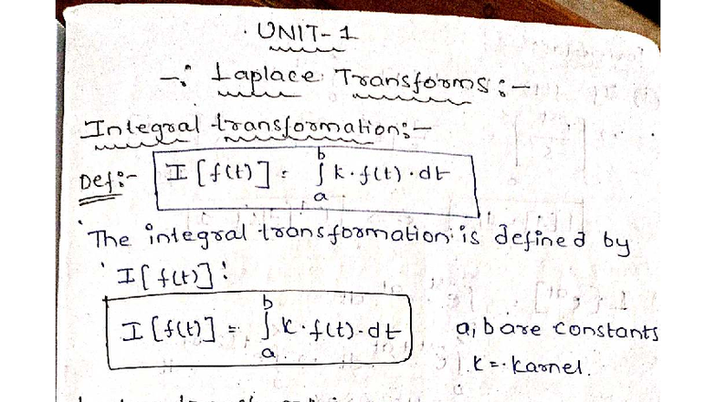
The Laplace transform converts a function of time, typically denoted as \( f(t) \), into a complex function of variable \( s \), written as \( F(s) \). Formally, defined for functions \( f(t) \) that are piecewise continuous and of exponential order, the transform is expressed as: \[ \mathcal{L}\{f(t)\} = F(s) = \int_{0^{-}}^{\infty} f(t)e^{-st}\,dt \] This mathematical bridge converts differential equations—ubiquitous in physical modeling—into algebraic formulations, simplifying operations such as differentiation and integration into straightforward multiplications. As Dr.
Eleanor Finch, applied mathematician at the Institute of Advanced Engineering, explains: “The real power of the Laplace transform is its ability to turn dynamic problems into spectral ones, where frequency responses reveal system stability and performance.”
For engineers and physicists, the ability to switch between domains is indispensable. The frequency-domain perspective unlocks critical insights: resonant frequencies, transient responses, and system stability—all of which are hidden beneath the surface in the time domain. The Table of Laplace Transforms codifies this connection, providing instant access to known transforms and their inverse counterparts, enabling rapid analysis across domains.
Core Structure of the Table of Laplace Transforms
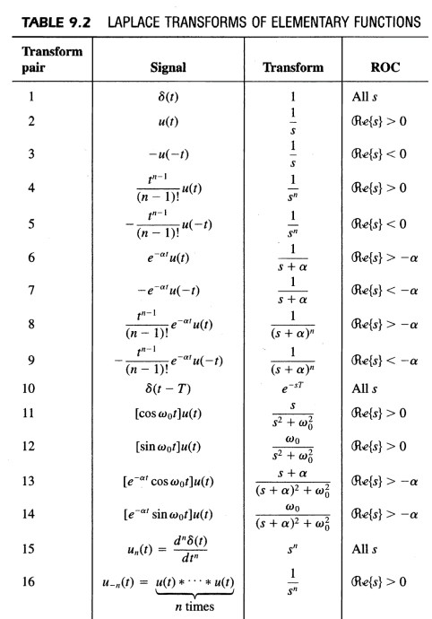
The Table of Laplace Transforms serves as a centralized, systematic reference—organized by standard function families such as exponentials, trigonometric functions, polynomials, and decaying exponentials. Its layout allows users to quickly identify transform pairs without re-deriving every result. Major elements include:
Basic Exponential Functions: \( \mathcal{L}\{e^{at}\} = \frac{1}{s - a} \), fundamental for modeling decay and growth processes in circuits and mechanics.
Polynomials and Shifts: \( \mathcal{L}\{t^n\} = \frac{n!}{s^{n+1}}, \quad \mathcal{L}\{f(t - a)u(t - a)\} = e^{-as}F(s) \), enabling analysis of rise times and time-delayed responses.
Standard Laplace Pairs: The table catalogs inverse transforms, including units from physics: impulse response, step response, and decay physiology in control systems.
This systematic indexing empowers engineers to cast complex differential equations—such as \( \frac{dy}{dt} + 3y = u(t) \)—into algebraic forms \( sY(s) - y(0) + 3Y(s) = \frac{1}{s} \), solvable via algebraic manipulation and partial fraction decomposition.
Key Transform Families and Their Engineering Significance
The Table of Laplace Transforms emphasizes several canonical pairs central to engineering analysis:
Exponential Growth/Decay: The transform \( \mathcal{L}\{e^{-at}\} = \frac{1}{s + a} \) models battery discharge or radioactive decay—phenomena critical in energy systems. “Understanding decay via Laplace transforms clarifies how quickly stored energy dissipates,” notes Dr. Marcus Reed, control systems specialist at MIT.
Step Function Response: \( \mathcal{L}\{u(t)\} = \frac{1}{s} \) captures idealized sudden inputs, forming the basis for step responses that reveal stability and transient behavior in feedback systems.
Unit Impulse Delta: The Dirac delta, with \( \mathcal{L}\{\delta(t - a)\} = e^{-as} \), encodes instantaneous inputs—pivotal for impulse testing and system identification.
Trigonometric Oscillations: Transforms like \( \mathcal{L}\{\sin(\omega t)\} \) underpin analysis of electrical filters, mechanical vibrations, and signal modulation, where frequency domain insight dramatically enhances design precision.
Exponential Multiplication (Tau Shift): Pairs such as \( \mathcal{L}\{e^{-at}u(t)\} = \frac{1}{s + a} \) translate time delays into exponential damping, essential for modeling signal propagation and control lags.
These families bridge theory and application—turning abstract equations into actionable data.
For instance, a mechanical vibration system with damping modeled as \( un'(t) + cu(t) = 0 \) transforms via \( s(s + c/m)U(s) = 0 \), revealing poles at \( s = 0 \) and \( s = -c/m \)—directly indicating stable, exponentially damped motion.